Demo Stereo

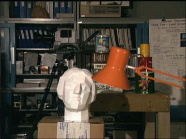
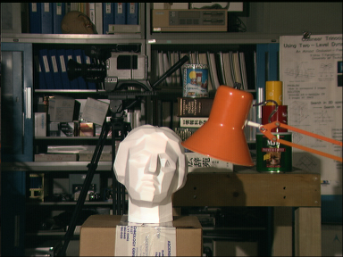
Estimating the disparity field between two stereo images is a common task in computer vision, e.g., to determine a dense depth map. Please refer to the Chapter 1 of the Master Thesis 3D Map Reconstruction with Variational Methods for introduction to disparity field estimation. Evaluation and qualitative comparison of a large number of different algorithms for disparity field estimation may be found at vision.middlebury.edu web-site. In this tutorial we show how to develop a probabilistic model for evaluation a high-quality disparity field between two stereo images.

Input stereo pair			Output
tsukuba_left.jpg	tsukuba_right.jpg		Resulting Disparity Map

We start this tutotial in the same way as Demo Train or Demo Dense tutorials: with reading the command line arguments and initializing basic DGM classes. Our primary input data here is the couple of stereo images: imgL and imgR. We also represent disparity as integer shift value in pixels: the distance in x-coordinate-direction between the same pixel in left and right images. Every possible diparity value between given minDisparity and maxDisparity is the class label (state) with its own probability.

#include "DGM.h"
using namespace DirectGraphicalModels;

int main(int argc, char *argv[])
{
    if (argc != 5) {
        print_help(argv[0]);
        return 0;
    }

    // Reading parameters and images
    Mat       imgL          = imread(argv[1], 0);   if (imgL.empty()) printf("Can't open %s\n", argv[1]);
    Mat       imgR          = imread(argv[2], 0);   if (imgR.empty()) printf("Can't open %s\n", argv[2]);
    int       minDisparity  = atoi(argv[3]);
    int       maxDisparity  = atoi(argv[4]);
    int       width         = imgL.cols;
    int       height        = imgL.rows;
    unsigned int nStates    = maxDisparity - minDisparity;

    CGraphPairwiseKit graphKit(nStates, INFER::TRW);

Please note, that in this tutorial we use pairwise graphical model with edges connection every node with its four direct neighbors. You can easily change to complete (dense) graphical model

by changing the factory DirectGraphicalModels::CGraphPairwiseKit to DirectGraphicalModels::CGraphDenseKit. The optimal parameters for the dense edge model may be optained using Demo Parameters Estimation.

Next we build a 2D graph grid and add a default edge model:

graphKit.getGraphExt().buildGraph(imgL.size());
graphKit.getGraphExt().addDefaultEdgesModel(1.175f);

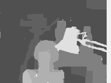
The most tricky part of this tutorial is to fill the graph nodes with potentials. We do not train any node potentials model, but estimate the potentials directly from the images using the formula: \( p(disp) = 1 - \frac{\left|imgL(x, y) - imgR(x + disp, y)\right|}{255} \), where \( disp \in \left[minDisp; maxDisp \right) \). This will give the highest potentials for those dosparities where the pixel values in left and right images nearly the same.

// ==================== Filling the nodes of the graph ====================
Mat nodePot(nStates, 1, CV_32FC1);                                      // node Potential (column-vector)
size_t idx = 0;
for (int y = 0; y < height; y++) {
    byte * pImgL    = imgL.ptr<byte>(y);
    byte * pImgR    = imgR.ptr<byte>(y);
    for (int x = 0; x < width; x++) {
        float imgL_value = static_cast<float>(pImgL[x]);
        for (unsigned int s = 0; s < nStates; s++) {                    // state
            int disparity = minDisparity + s;
            float imgR_value = (x + disparity < width) ? static_cast<float>(pImgR[x + disparity]) : imgL_value;
            float p = 1.0f - fabs(imgL_value - imgR_value) / 255.0f;
            nodePot.at<float>(s, 0) = p * p;
        }

        graphKit.getGraph().setNode(idx++, nodePot);
    } // x
} // y

Now to improve the result of stereo estimation we run inference and decoding.

You can check how the results look like without inference. To do so set the number of iterations to zero: i.e. use "decode(0)". This will be the resulting disparity field achieved

without application of the CRFs.

// =============================== Decoding ===============================
Timer::start("Decoding... ");
vec_byte_t optimalDecoding = graphKit.getInfer().decode(100);
Timer::stop();

And with some more efforts we convert the decoding results into a disparity field:

    // ============================ Visualization =============================
    Mat disparity(imgL.size(), CV_8UC1, optimalDecoding.data());
    disparity = (disparity + minDisparity) * (256 / maxDisparity);
    medianBlur(disparity, disparity, 3);

    imshow("Disparity", disparity);

    waitKey();

    return 0;
}