Chain

In this demo we consider more complex problem involving the chain of nodes. Such a problem is common in Markov chains and hidden Markov models These models may incorporate large graphs, what prevents from using brute-force exact decoding and inference algorithms. Nevertheless, we can take an advantage of the conditional independence properties induced by the chain structure and use polynomial-time exact message-passing inference algorithm. This example copies the idea from the Computer Science Graduate Careers

In order to run this demo, please execute "Demo 1D.exe" chain command

Building The Markov Chain

We build a chain, consisting of 60 nodes, which represents 60 years. Every node has 7 states and the first, initial node will have the potential: \((0.3, 0.6, 0.1, 0, 0, 0, 0)^\top\), whereas all other nodes are initiated with uniform distribution: \((\frac{1}{7}, \frac{1}{7}, \frac{1}{7}, \frac{1}{7}, \frac{1}{7}, \frac{1}{7}, \frac{1}{7})^\top\). We connect all nodes into a chain with undirected arcs:

using namespace DirectGraphicalModels;

const byte   nStates = 7;               // {grad scool, industry, video games, industry (with PhD), academia, video games (with PhD), deceased}
const size_t nNodes = 60;               // sixty years

CGraphPairwise  graph(nStates);

Mat nodePot = getNodePot();
graph.addNode(nodePot);                 // add the first node
nodePot.setTo(1.0f  / nStates);         // uniform distribution
for (size_t i = 1; i < nNodes; i++) 
    graph.addNode(nodePot);             // add nodes

Mat edgePot = getEdgePot();
for (size_t i = 0; i < nNodes - 1; i++) 
    graph.addArc(i, i + 1, edgePot);    // add arcs

The edge potential matrix is represented here as a transition matrix:

from\to	st.0	st.1	st.2	st.3	st.4	st.5	st.6
st.0	0.08	0.90	0.01	0	0	0	0.01
st.1	0.03	0.95	0.01	0	0	0	0.01
st.2	0.06	0.06	0.75	0.05	0.05	0.02	0.01
st.3	0	0	0	0.30	0.60	0.09	0.01
st.4	0	0	0	0.02	0.95	0.02	0.01
st.5	0	0	0	0.01	0.01	0.97	0.01
st.6	0	0	0	0	0	0	1

e.g. a probability of switching from state 3 at year i to state 5 at year i + 1 is 0.09. The node and edge potentials are returned with functions getNodePot() and getEdgePot() respectively.

Inference

The number of all possible configurations for our chain is equal to \(7^{60}\approx 5.08\times 10^{50}\), and it is not feasible to calculate joint probabilities for all of these configurations. Nevertheless, DGM has exact inference method for chains DirectGraphicalModels::CInferChain, which is based on a message-passing algorithm with the total cost of evaluating the marginals of \(O(nNodes\cdot nStates^2)\):

using namespace DirectGraphicalModels;

CInferChain inferer(graph);

inferer.infer();

Results

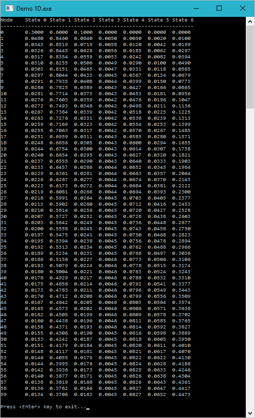
Finally, we depict the results of inference. Please note, that the marginal probability for the first node is equal to the initial probability: