Exact

In this demo, we use a very simple graphical model to represent a very simple probabilistic scenario, show how to input the model into DGM, and perform inference and decoding in the model. This example copies the idea from the Cheating Students Scenario

In order to run this demo, please execute "Demo 1D.exe" exact command

Building The Graphical Model

First of all we build a graph, consisting of 4 nodes, which represents 4 studens. We connect these nodes with undirected arcs. Since every student may give either true or false answer, every graph node will have 2 states:

using namespace DirectGraphicalModels;

const byte   nStates = 2;                                               // {false, true}
const size_t nNodes  = 4;                                               // four students

CGraphPairwise graph(nStates);

for (size_t i = 0; i < nNodes; i++)     graph.addNode();                // add nodes
for (size_t i = 0; i < nNodes - 1; i++) graph.addArc(i, i + 1);         // add arcs

Next we fill the potentials of nodes and arcs of the graph. We assume that four studens are sitting in a row, and even studens have 25% chance to answer right, whereas odd students have 90% chance. The edge potential describes that two neighbouring students are more likely to give the same answer. We fill the potentials by hand in the fillGraph() function:

Mat nodePot(nStates, 1,       CV_32FC1);                                // node Potential (column-vector)
Mat edgePot(nStates, nStates, CV_32FC1);                                // edge Potential (matrix)

// Setting the node potentials
for (size_t i = 0; i < nNodes; i++) {
    if (i % 2) {                                                        // for odd nodes
        nodePot.at<float>(0, 0) = 0.10f;                                // nodePot = (0.10; 0.90)^T
        nodePot.at<float>(1, 0) = 0.90f;    
    } else {                                                            // for even nodes
        nodePot.at<float>(0, 0) = 0.75f;                                // nodePot = (0.75; 0.25)^T
        nodePot.at<float>(1, 0) = 0.25f;    
    }
    graph.setNode(i, nodePot);
}

// Defying the edge potential matrix
edgePot.at<float>(0, 0) = 2.0f; edgePot.at<float>(0, 1) = 1.0f;
edgePot.at<float>(1, 0) = 1.0f; edgePot.at<float>(1, 1) = 2.0f;

// Setting the edge potentials
for (size_t i = 0; i < nNodes - 1; i++) 
    graph.setArc(i, i + 1, edgePot);

We end up with the followiung graphical model:

The initial chances for students to give right ansvers, were given as if every student was alone. Now, when we have all four students sitting together (modelled with edge potentials), these chances are not independent anymore. We are interested in the most probable scenario, how answer these students, when they answer together. To solve this problem, we have to apply decoding or/and inference upon the given graph. Let us consider these processes separately.

Decoding

The decoding task is to find the most likely configuration, i.e. the configuration with the highest joint probability.

For trivial graphs where it is feasible to enumerate all possible configurations, wich is equal to \(nStates^{nNodes}\), we can apply exact decoding - for other cases, approximate approaches should be used. Exact decoding is based on brute force estimation of the joint probabilities for every possible configuration of random variables, associated with the graph nodes. In DGM decoding returns the most likely configuration directly:

using namespace DirectGraphicalModels;

CDecodeExact decoderExcact(graph);

vec_byte_t decoding_decoderExcact = decoderExcact.decode();

Inference

The inference task is to find the marginal probabilities of individual nodes taking individual states.

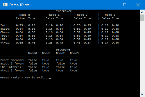
For our example, marginal probabilities describe the chance of every student to answer the question right. DGM inference procedures store the marginal probabilities in the node potentials vectors.

using namespace DirectGraphicalModels;

CInferExact infererExact(graph);

infererExact.infer();                                           // changes the node potentials

Each inference class has decode() function and could be used for approximate decoding. This function returns the configuration, which maximases the marginals, and this configuration in general is not the same as the configuration corresponding to the highest joint probability, i.e DirectGraphicalModels::CDecodeExact::decode() \(\neq\) DirectGraphicalModels::CInferExact::decode():

vec_byte_t decoding_infererExcact = infererExact.decode();      // approximate decoding from inferer

Results

Finally, we depict the results of inference and decoding. In the INFERENCE table the initial node potentials, and marginal probabilities after inferece are shown (for our simple graph, we can also use exact chain and tree inference algorithms, approximate loopy belief propagation and viterbi algorithms). In the DECODING table the rsults of the exact decoding and approximate decodings from inferece are shown. Please note, that the correct configuration, provided by the exact decoder is {false, true, true, true}. However, the exact inference methods provide us with the configuration {false, true, false, true}, and only Viterbi (max-product message passing algorithm) gives correct decoding, build upon marginals from the table INFERENCE: