Demo Visualization

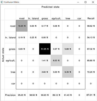
DGM library has a rich set of tools for visualizing the data, intermediate and final results, as well as for interaction with created figures. It also provides tools for analyzing the classification accuracy. In this example we took the Demo Train tutorial, simplified the training sections and expanded the visulaization part. First we estimate the quality of classification with confusion matrix, then we visualize the feature distributions for defined classes in the training dataset as well as the node and edge potentials. For user interaction capacity we define additional functions for handling the mouse clicks over the figures.

Confusion matrix	Edge potential matrix	Node potential vector	Feature distribution histograms

#include "DGM.h"
#include "VIS.h"
using namespace DirectGraphicalModels;
using namespace DirectGraphicalModels::vis;

struct USER_DATA {
    CGraphPairwise      & graph;
    CMarkerHistogram    & marker;
    int                   imgWidth;
    USER_DATA(CGraph &_graph, CMarkerHistogram &_marker, int _imgWidth) : graph(static_cast<CGraphPairwise&>(_graph)), marker(_marker), imgWidth(_imgWidth) {}
};

int main(int argc, char *argv[])
{
    const Size  imgSize     = Size(400, 400);
    const int   width       = imgSize.width;
    const int   height      = imgSize.height;
    const byte  nStates     = 6;                // {road, traffic island, grass, agriculture, tree, car}        
    const word  nFeatures   = 3;        

    if (argc != 4) {
        print_help(argv[0]);
        return 0;
    }

    // Reading parameters and images
    Mat img = imread(argv[1], 1); resize(img, img, imgSize, 0, 0, INTER_LANCZOS4);      // image
    Mat fv  = imread(argv[2], 1); resize(fv,  fv,  imgSize, 0, 0, INTER_LANCZOS4);      // feature vector
    Mat gt  = imread(argv[3], 0); resize(gt,  gt,  imgSize, 0, 0, INTER_NEAREST);       // groundtruth

    CTrainNodeBayes         nodeTrainer(nStates, nFeatures);
    CTrainEdgePottsCS       edgeTrainer(nStates, nFeatures);
    vec_float_t             vParams = {400, 0.001f};
    auto                    graphKit = CGraphKit::create(GraphType::pairwise, nStates);

    // Define custom colors in RGB format for our classes (for visualization)
    vec_nColor_t          palette;
    palette.push_back(std::make_pair(CV_RGB(64,  64,   64), "road"));
    palette.push_back(std::make_pair(CV_RGB(0,  255,  255), "tr. island"));
    palette.push_back(std::make_pair(CV_RGB(0,   255,   0), "grass"));
    palette.push_back(std::make_pair(CV_RGB(200, 135,  70), "agricult."));
    palette.push_back(std::make_pair(CV_RGB(64,  128,   0), "tree"));
    palette.push_back(std::make_pair(CV_RGB(255,   0,   0), "car"));
    // Define feature names for visualization
    vec_string_t        featureNames    = {"NDVI", "Var. Int.", "Saturation"};
    CMarkerHistogram    marker(nodeTrainer, palette, featureNames);
    CCMat               confMat(nStates);

    // =============================== Training ================================
    Timer::start("Training... ");
    nodeTrainer.addFeatureVecs(fv, gt);                                     // Only Node Training
    nodeTrainer.train();                                                    // Contrast-Sensitive Edge Model requires no training
    Timer::stop();

    // ==================== Building and filling the graph =====================
    Timer::start("Filling the Graph... ");
    graphKit->getGraphExt().setGraph(nodeTrainer.getNodePotentials(fv));
    graphKit->getGraphExt().addDefaultEdgesModel(fv, 400);
    Timer::stop();

    // ========================= Decoding =========================
    Timer::start("Decoding... ");
    vec_byte_t optimalDecoding = graphKit->getInfer().decode(10);
    Timer::stop();

    // ======================== Evaluation ======================== 
    Mat solution(imgSize, CV_8UC1, optimalDecoding.data());
    confMat.estimate(gt, solution);                                         // compare solution with the groundtruth
    char str[255];
    sprintf(str, "Accuracy = %.2f%%", confMat.getAccuracy());
    printf("%s\n", str);

    // ====================== Visualization =======================
    marker.markClasses(img, solution);
    rectangle(img, Point(width - 160, height- 18), Point(width, height), CV_RGB(0,0,0), -1);
    putText(img, str, Point(width - 155, height - 5), FONT_HERSHEY_SIMPLEX, 0.45, CV_RGB(225, 240, 255), 1, LineTypes::LINE_AA);
    imshow("Solution", img);
    
    // Feature distribution histograms
    marker.showHistogram();

    // Confusion matrix
    Mat cMat    = confMat.getConfusionMatrix();
    Mat cMatImg = marker.drawConfusionMatrix(cMat, MARK_BW);
    imshow("Confusion Matrix", cMatImg);

    // Setting up handlers
    USER_DATA userData(graphKit->getGraph(), marker, width);
    setMouseCallback("Solution",  solutiontWindowMouseHandler, &userData);

    waitKey();

    return 0;
}

Mouse Handler for drawing the node and edge potentials
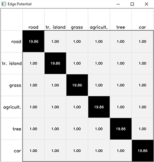
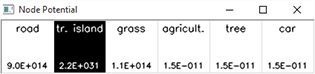
This mouse handler provides us with the capacity of user interaction with the Solution window. By clicking on the pixel of the solution image, we can derive the node potential vector from the graph node, associated with the chosen pixel, and visualize it. In this example, each graph node has four edges, which connect the node with its direct four neighbors; we visualize one edge potential matrix, corresponding to one of these four edge potentials. The visualization of the node and edge potentials helps to analyze the local potential patterns.

void solutiontWindowMouseHandler(int Event, int x, int y, int flags, void *param)
{
    USER_DATA   * pUserData = static_cast<USER_DATA *>(param);
    if (Event == MouseEventTypes::EVENT_LBUTTONDOWN) {
        Mat           pot, potImg;
        size_t        node_id   = pUserData->imgWidth * y + x;

        // Node potential
        pUserData->graph.getNode(node_id, pot);
        potImg = pUserData->marker.drawPotentials(pot, MARK_BW);
        imshow("Node Potential", potImg);

        // Edge potential
        vec_size_t child_nodes;
        pUserData->graph.getChildNodes(node_id, child_nodes);
        if (child_nodes.size() > 0) {
            pUserData->graph.getEdge(node_id, child_nodes.at(0), pot);
            potImg = pUserData->marker.drawPotentials(pot, MARK_BW);
            imshow("Edge Potential", potImg);
        }

        pot.release();
        potImg.release();
    }
}

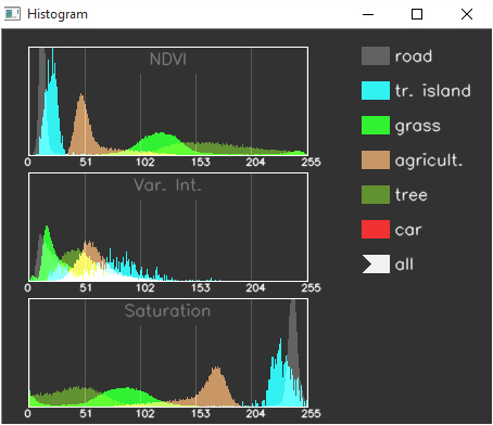
Mouse Handler for drawing the feature distribution histograms
This mouse handler allows for user interaction with Histogram window. Its capable to visualize the feature distributions separately for each class. User can chose the needed class by clicking on the color box near to the class name. These feature distributions allow for analyzing the separability of the classes in the feature sapce.

Starting from the version 1.5.1 this mouse handler is built in the VIS module. Thus, no extra code is needed.