Efficient K-Nearest Neighbours
The K-nearest neighbours classifier (KNN) is a type of instance-based learning, or lazy learning, where the function is only approximated locally and all computation is deferred until classification. Thus, the KNN approach is among the simplest of all discriminative approaches, but this classifier is still especially effective for low-dimensional feature spaces. However, the application of the KNN model in practical applications is problematic because of its low-speed performance for large datasets represented in high-dimensional feature spaces and for the large number of neighbors – K. In this article we address exactly this problem of the KNN model.
The input for the KNN algorithm consists of the K closest training samples in the feature space and the output is a class label l. An observation (or testing sample) y is classified by a majority vote of its neighbours, with the observation being labelled by the class most common among its K nearest neighbours (see figure below, center). In case of K = 1 the class of that single nearest neighbour is simply assigned to the observation y.
-

- The original distributions of 160'000 samples from the dataset
-

- Resulting k-Nearest Neighbors decision map
-

- k-Nearest Neighbors classifier
In order to estimate the potentials we consider the class of every neighbour as a vote for the most likely class of the observation. If the number of neighbours, having class l is Kl we can define the probability of the association potentials as: (see figure above, right)
=frac{K_l}{K}")
It can be useful to assign weight to the contributions of the neighbors, so that the nearer neighbors contribute more to the average than the more distant ones. For example, a common weighting scheme consists in giving each neighbor a weight of 1 / r, where r is the distance to the neighbor. For our weighting scheme we modify this idea as follows: let r will be the Euclidean distance from the test sample to the nearest training sample in feature space and ri – Euclidean distance to every found neighbor. Then we can rewrite the previous equation with weighting coefficient:
=frac{1}{K}sum_i{frac{1_l}{(1+r_i-r)^2}},")
where 1l means 1 if the class of the training sample is l and 0 otherwise.
Optimization
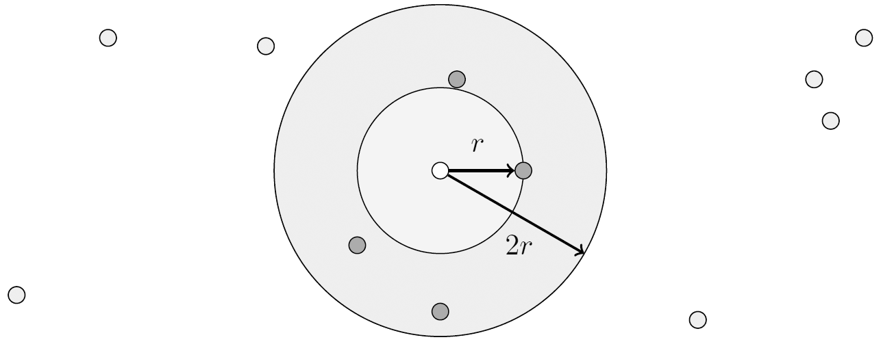
The search algorithm aims usually to find exactly K nearest neighbors. However it may happen, that distant neighbors do not affect probability p(x = l|y) much. For example, the nearest neighbor with ri = r contributes value of 1 / K to the probability. And a neighbor, twice as distant from the testing sample (ri = 2r) will contribute only 1 / K(1 + r)2. For the optimization purpose we stop the search once the distance from the test sample to the next nearest neighbor exceeds 2r. Thus, only K’ ≤ K neighbors in area enclosed between two spheroids of radii r and 2r are considered (see figure below) and weighted according to the equation: p(x = l|y) = Kl / K’.
The neighbors are taken from a set of objects for which the class is known. This can be thought of as the training set for the algorithm, though no explicit training step is required. A peculiarity of the KNN algorithm is that it is sensitive to the local structure of the data.
Evaluation
Our implementation of the KNN model in DGM C++ library is based on the KD-tree data structure, which is used to store points in k-dimensional space. Leafs of the KD-tree store feature vectors with corresponding groundtruth and every such feature vector is stored in one and only one leaf. Tree nodes correspond to axis-oriented splits of the space. Each split divides space and dataset into two distinct parts. Subsequent splits from the root node to one of the leafs remove parts of the dataset until only small part of the dataset (a single feature vector) is left.
KD-trees allow to efficiently perform searches “K nearest neighbors of N”. Considering number of dimensions k fixed, and dataset size N training samples, the time complexity for building a KD-tree is O(N · logN) and for finding K nearest neighbors – close to O(K · logN). However, its efficiency decreases as dimensionality k grows, and in high-dimensional spaces KD-trees give no performance over naive O(N) linear search.
In order to evaluate the performance of our KNN model, we perform a number of experiments: 2r-KNN, 4r-KNN, 8r-KNN, 16r-KNN and 32r-KNN – models, where the nearest neighbors enclosed between two spheroids of radii r and 2r (4r, 8r, 16r and 32r respectively) are only taken into account. In the ∞r-KNN experiment all the K neighbors were considered. And finally the KNN experiment is the OpenCV implementation of KNN (CvKNN) based on linear search. The overall accuracies and the timings for all 7 experiments are given in table below:
| 2r-KNN | 4r-KNN | 8r-KNN | 16r-KNN | 32r-KNN | ∞r-KNN | CvKNN | |
|---|---|---|---|---|---|---|---|
| Training: | 4659 sec | 4659 sec | 4659 sec | 4659 sec | 4659 sec | 4659 sec | 102 sec |
| Classification: | 8,3 sec | 22,2 sec | 52,8 sec | 97,2 sec | 134,9 sec | 216,1 sec | 45,3 sec |
| Accuracy: | 81,39 % | 81,65 % | 81,97 % | 82,11 % | 82,33 % | 82,42 % | 82,36 % |
Accuracies and timings for Intel® Core™ i7-4820K CPU with 3.70 GHz required for training on 1016 scenes and classification of 1 scene.
Our 2r-KNN model gives almost the same overall accuracies as the reference KNN model, but needs almost 5.5 times less time. The training time of the xr-KNN models, which includes the building of the KD-tree, takes 78 minutes, what is much more slower then 1,7 minutes for KNN training. However, the training in practical applications is performed only once and could be done offline, when the classification time is more critical for the whole classification engine performance. In the table above we can also observe almost linear increase of the classification time with increasing the outer spheroid radius to 4r, 8r, etc. Figure below shows the classification results for the experiments 2r-KNN – ∞r-KNN.
-

- 2r-KNN
-

- 4r-KNN
-

- 8r-KNN
-

- 16r-KNN
-

- 32r-KNN
-

- ∞r-KNN
April 21, 2020 @ 23:53
Your mode of telling all in this article is really good, every one be able to
easily know it, Thanks a lot.
May 19, 2020 @ 15:06
Hurrah! At last I got a website from where I
be capable of genuinely take useful data concerning my study and knowledge.